Filtered CoCluster Correlation Network Creation Guide
Nagashree Avabhrath, Mikhail Bailey, Mark Grimes, Madison Moffett, Grant Smith
CoClusterCorrelationNetwork.RmdThis Package
The CCCN_CFN package takes experimental data of post-translational modifications based on experimental conditions and generates clusters of likely pathways. These pathways are generated based on analysis of which ptms cluster together (in their ptms based on the same environmental conditions) compared to how those proteins are known to interact (using the STRINGdb database).
An important note about this package: there are no returned outputs from any of the functions. All outputs listed are assigned to the Global Namespace in order to prevent loss of data and promote ease of use. Some functions also pull variables from the global namespace. Ensure that all data is loaded into the global environment especially if analysis is completed across multiple sessions.
This File
This vignette is intended to be a step-by-step guide to walk users through the process of using the CCCN_CFN package. It includes an example pipeline demonstrating how to run the full analysis along with descriptions of each function. this pipeline must be run in order as subsequent steps require the data produced in previous steps. Estimated run-times are included with each description and are based on a preliminary dataset of ~9,000 post-translational modifications and 70 experimental conditions processed with a 12th Gen i5 processor and 8GB of RAM.
Pipeline
Step 1: Make Cluster List
Code
MakeClusterList(ptmtable, correlation.matrix.name = "ptm.correlation.matrix", list.name = "clusters.list", toolong = 3.5)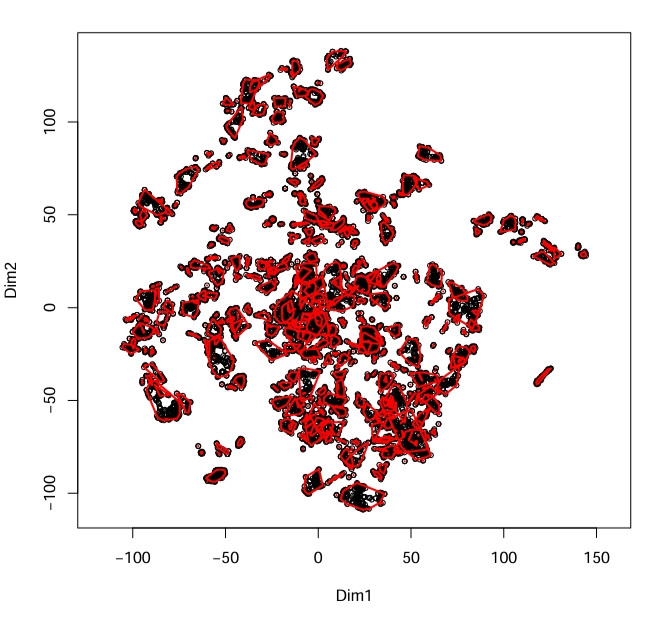
Figure 1 Example plot produced by MakeClusterList
calculated using Euclidean Distance
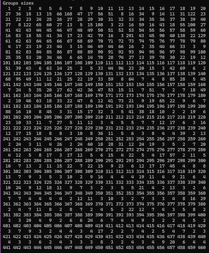
Figure 2 Output of MakeClusterList
#> $`1`
#>                                             PTM.Name group
#> 1                                      AARS ubi K747     1
#> 2                                    ANAPC5 ubi K289     1
#> 3                                      CUTA ubi K112     1
#> 4                                     CYHR1 ubi K349     1
#> 5                                      EEF2 ack K498     1
#> 6                                       F11R ubi K97     1
#> 7                                        GMPS ack K9     1
#> 8                                      HERC2 ubi K20     1
#> 9                                     KPNB1 ubi K541     1
#> 10                                     LASP1 ubi K59     1
#> 11                                     LNPEP ubi K32     1
#> 12                                    MRPS27 ubi K94     1
#> 13                                      NME1 ack K39     1
#> 14                                     PCNA ubi K110     1
#> 15                                      PKM ack K141     1
#> 16                                     PLAU ubi K403     1
#> 17                                     PLK1 ubi K492     1
#> 18                                   PNPLA2 ubi K435     1
#> 19                                    PSMC1 ubi K237     1
#> 20                                    RBCK1 ubi K342     1
#> 21                                    RPS15A ubi K12     1
#> 22                                    TCAF1 ubi K817     1
#> 23 TUBB4B ubi K379; TUBB2A ubi K379; TUBB2B ubi K379     1
#> 24                                    UIMC1 ubi K245     1
#> 25                                     USP5 ubi K318     1
#> 26                                    VAMP7 ubi K125     1
#> 27                                      VCP ubi K295     1
Figure 3 First cluster created by Euclidean Distance
Description
Make Cluster List is the first step in the analyzing one’s data. This function takes the post-translational modification table and runs it through three calculations of distance: Euclidean Distance, Spearman Dissimilarity (1 - |Spearman Correlation|), and the average of the two of these. These calculations find the ‘distance’ between ptms based upon under what conditions they occur. These matricies are then run through t-SNE in order to put them into a 3-dimensional space. Please note: t-SNE involves an element of randomness; in order to get the same results, set.seed(#) must be called. A correlation table is also produced based on the Spearman Correlation table.
Input
- ptmtable
- A data frame of post-translational modifications. Formatted with
numbered rows and the first column containing PTM names. The rest of the
column names should be drugs (experimental conditions). Values of the
table are numeric values that represent how much the PTM has reacted to
the drug.
- A data frame of post-translational modifications. Formatted with
numbered rows and the first column containing PTM names. The rest of the
column names should be drugs (experimental conditions). Values of the
table are numeric values that represent how much the PTM has reacted to
the drug.
- correlation.matrix.name
- Desired name for the correlation matrix to be saved as; defaults to
ptm.correlation.matrix
- Desired name for the correlation matrix to be saved as; defaults to
ptm.correlation.matrix
- list.name
- Desired name for the lists of clusters to be saved as; defaults to
clusters.list
- Desired name for the lists of clusters to be saved as; defaults to
clusters.list
- toolong
- Threshold for cluster separation; defaults to 3.5
Output
- ptm.correlation.matrix (or otherwise named by
correlation.matrix.name)
- A data frame showing the correlation between ptms (as the rows and
the columns). NAs are placed along the diagonal
- A data frame showing the correlation between ptms (as the rows and
the columns). NAs are placed along the diagonal
- clusters.list (or otherwise named by list.name)
- A list of three-dimensional data frames used to represent ptms in space to show relationships between them based on distances. Based on Euclidean Distance, Spearman Dissimilarity, and SED (the average between the two)
Step 2: Make Correlation Network
Code
MakeCorrelationNetwork(tsne.matrices, ptm.correlation.matrix, keeplength = 2, common.clusters.name = "common.clusters", cccn.name = "cccn_matrix")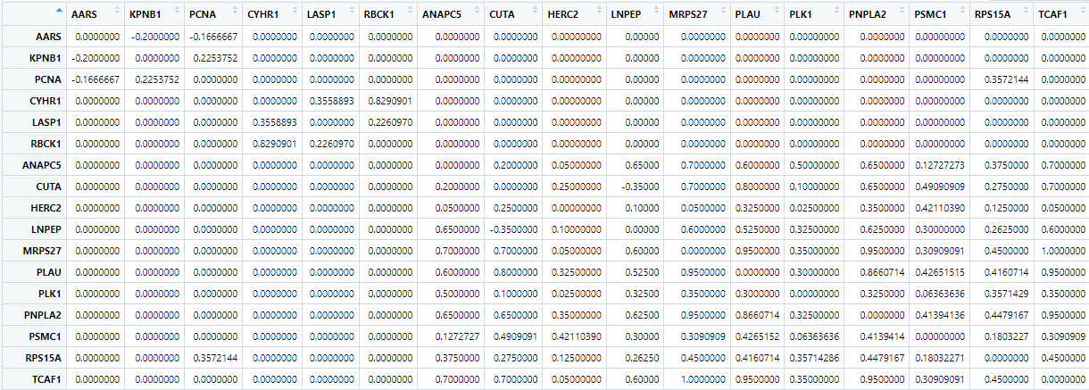
Figure 4 First 17 rows and columns of the cccn_matrix
produced by MakeCorrelationNetwork
Description
Make Correlation Network first finds the intersection between the Euclidian, Spearman, and SED cluster matrices in order to find the intersection between the three groups. It then adds the Genes in these PTMs to a list of common clusters and turns it into an adjacency matrix. This adjacency matrix is used to filter relevant data — clusters — from the Spearman correlation matrix. The resultant cocluster correlation network shows strength of relationships between proteins using the common clusters between the three distance metrics.
Input
- clusters.list
- A list of three-dimensional data frames used to represent ptms in
space to show relationships between them based on distances. Based on
Euclidean Distance, Spearman Dissimilarity, and SED (the average between
the two)
- A list of three-dimensional data frames used to represent ptms in
space to show relationships between them based on distances. Based on
Euclidean Distance, Spearman Dissimilarity, and SED (the average between
the two)
- ptm.correlation.matrix
- A data frame showing the correlation between ptms (as the rows and the columns). NAs are placed along the diagonal.
- keeplength
- MakeClusterList only saves subsets whose size is strictly greater than keeplength; defaults to 2
- example: [‘AARS’, ‘ABR’] will be discarded unless keeplength < 2
- common.clusters.name
- Desired name for the common clusters output; defaults to
common.clusters
- Desired name for the common clusters output; defaults to
common.clusters
- cccn.name
- Desired name for the cocluster combined network matrix; defaults to cccn.matrix
Output
- common.clusters (or otherwise named by common.clusters.name)
- The list of common clusters between all three distance metrics (Euclidean, Spearman, and SED)
- cccn.matrix (or otherwise named by cccn.name)
- A matrix showing strength of relationships between proteins using common clusters between the three distance metrics
Step 3: Retrieve Database Edgefiles
Description
PPI (protein-protein interaction) databases are consulted in order to filter the clusters by proteins that are known to interact with each other as well as how strongly they are known to interact. The standard PPI database that is used is STRINGdb, and getting data from this database is the first step. This is accomplished with the function GetSTRINGdb. Please note, however, that the user may consult any database that they choose. After getting STRINGdb data (or not), the user runs MakeDBInput which produces a text file of all of their gene names. This information can be copy and pasted into any database that the user chooses in order to get other PPI networks. Step three is getting a GeneMANIA network, which is also optional but recommended. The user pastes their input data into GeneMANIA on the Cytoscape app and saves the edgefile and the nodetable. These files are then input into ProcessGMEdgefile in order to sort the data.
Note again that the database input can be used in any PPI database that the user chooses, though this package only explicitly supports STRINGdb and GeneMANIA. If another database is chosen, its file will have to be filtered manually by the user before moving on to step 4. The file should have three columns. Column one and two should strictly be labeled “Gene.1” and “Gene.2” in order to integrate with other PPI databases. The third column should contain the edgeweight and may be named however the user chooses. It is recommended, though, that the database is specified as well as the term ‘weight’ in the column name.
Part 1 — Get STRINGdb Data
Code
GetSTRINGdb(cccn_matrix, STRINGdb.name = "string.edges", nodenames.name = "nodenames")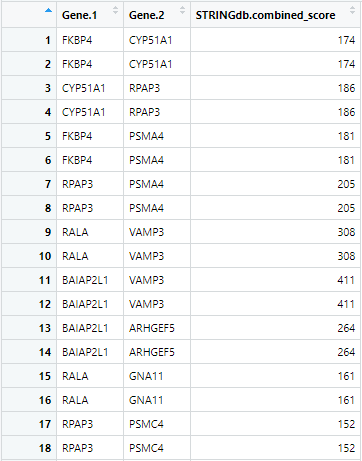
Figure 5 First 18 rows of string.edges produced by
GetSTRINGdb
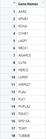
Figure 6 First 18 rows of nodenames produced by
GetSTRINGdb
Input
- cccn.matrix
- A matrix showing strength of relationships between proteins using
the common clusters between the three distance metrics
- A matrix showing strength of relationships between proteins using
the common clusters between the three distance metrics
- STRINGdb.name
- Desired name for STRINGdb data; defaults to string.edges
- Desired name for STRINGdb data; defaults to string.edges
- nodenames.name
- Desired name for list of gene names; defaults to nodenames
Part 2 — Get File for Database Input
Code
MakeDBInput(cccn_matrix, file.path.name = "db_nodes.txt")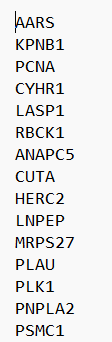
Figure 7 First 15 lines from the produced text file
Input
- cccn.matrix
- A matrix showing strength of relationships between proteins using
the common clusters between the three distance metrics
- A matrix showing strength of relationships between proteins using
the common clusters between the three distance metrics
- file.path.name
- Desired path for file to be saved as; defaults to db_nodes.txt
Part 3 — Process GeneMANIA File
Code
ProcessGMEdgefile(gm.edgefile.path, gm.nodetable.path, nodenames, gm.network.name = "gm.network")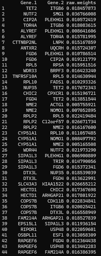
Figure 8 First 44 rows of the GeneMANIA network
Input
- gm.edgefile.path
- Path to the GeneMANIA edgefile
- gm.nodetable.path
- Path to the GeneMANIA nodetable
- db_nodes.path
- Path to the nodenames file created in make_db_input
- gm.network.name
- Desired name for the output of the GeneMANIA network, defaults to gm.network
Step 4: Build PPI Network
Code
BuildPPINetwork(cccn_matrix, db_file_paths = c(), ppi.network.name = "ppi.network")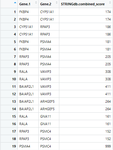
Figure 9 First 19 rows of the ppi_network produced by
find_ppi_edges
Description
Note: Examples take about 5-10 minutes to run.
Protein-Protein Interaction (or PPI) networks are networks that show us how different proteins are known interact with each other. STRINGdb — a database of these PPI networks — is automatically consulted along with any other database files that are generated and entered by the user. It then gathers data from the PPI networks and filters them down to only examine the determined genes of interest. The data from STRINGdb and any provided files are then combined and returned. The returned data frame shows how strongly the proteins are known to interact.
Input
- cccn_matrix
- A matrix showing strength of relationships between proteins using
the common clusters between the three distance metrics
- A matrix showing strength of relationships between proteins using
the common clusters between the three distance metrics
- db_file_paths (optional pre-step 3)
- A vector of paths to the additional ppi network files. This is
initialized to an empty vector
- A vector of paths to the additional ppi network files. This is
initialized to an empty vector
- gm.network (optional pre-step 3)
- GeneMANIA network produced in optional pre-step 3; defaults to
NA
- GeneMANIA network produced in optional pre-step 3; defaults to
NA
- ppi.network.name
- Desired name for the output of FindPPIEdges; defaults to ppi.network
Step 5: Cluster Filtered Network
Code
ClusterFilteredNetwork(cccn.matrix, ppi.network, cfn.name = "cfn")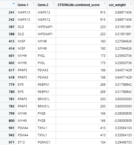
Figure 10 First 19 rows of the cfn produced by
ClusterFilteredNetwork
Description
Cluster Filtered Network checks all of the edges in the PPI network to see ensure that both of the genes are within our cocluster correlation network and that its weight is nonzero. If either of these conditions are not met, then it will be removed from the list of PPI edges. This new, cluster filtered network is then returned.
Input
- cccn.matrix
- A matrix showing strength of relationships between proteins using
the common clusters between the three distance metrics
- A matrix showing strength of relationships between proteins using
the common clusters between the three distance metrics
- ppi.network
- A dataframe representing how strongly proteins are known to
interact
- A dataframe representing how strongly proteins are known to
interact
- cfn.name
- Desired name for the output of ClusterFilteredNetwork; defaults to cfn
Step 6: Pathway Crosstalk Network
Code
PathwayCrosstalkNetwork(file = "bioplanet.csv", common.clusters, edgelist.name = "edgelist")Figure 11 Will exist at some point
Description
Note: This step is directory sensitive. You can check and set your directory in R using getwd() and setwd(“yourdirectoryhere”) respectively. It needs a path to the bioplanet file and will put an edgelist file in your working directory, or getwd(). If you cannot find a file, please check your directories first.
Pathway Crosstalk Network is the final step in the pipeline. It requires input of an external database, bioplanet, which consists of groups of genes (proteins) involved in various cellular processes. The PCN turns this database into a list of pathways and converts those pathways into a pathway x pathway edgelist that possesses multiple weights, a jaccard similarity and a score derrived from Cluster-Pathway Evidence using common clusters found in Make Correlation Network.
Input
- file
- File path for the pathway data from Bioplanet (can also take in a
data frame that is formatted correctly like the one found in the data
directory, but this is not recommended as formatting must match sample
data exactly)
- File path for the pathway data from Bioplanet (can also take in a
data frame that is formatted correctly like the one found in the data
directory, but this is not recommended as formatting must match sample
data exactly)
- common.clusters
- List of common clusters from MakeCorrelationNetwork
- List of common clusters from MakeCorrelationNetwork
- edgelist.name
- The desired name of the Pathway to Pathway edgelist file created. The PCN file will automatically add ‘.csv’ to the end for you. Intended for use in Cytoscape. Defaults to edgelist
Output
- edgelist (or otherwise named by edgelist.name)
- An edgelist file that is created in the working directory. It contains pathway source-target columns, with edge weights of their jaccard similarity and their Cluster-Pathway Evidence score. Info about the Cluster-Pathway Evidence score can be found at: https://journals.plos.org/ploscompbiol/article?id=10.1371/journal.pcbi.1010690